Fifteen Papers in Modern AI: Reading Notes by a Statistician
Before downloading, note that the notes are put together using LLMs. Claims about each paper were checked against the paper, and my interpretations are marked as such. I welcome corrections.
Download link: Fifteen Papers: Reading Notes (PDF)
These are my notes on fifteen papers that keep coming up when people discuss modern AI. They are short on purpose. For each paper: the problem, the core mathematics, what was actually shown, and how I read it as a statistician. The PDF has more detail.
Two habits run through the notes.
- Paper vs. me. Everything under Shown comes from the paper. Everything under My reading is my interpretation, and the paper may not say it.
- Claims stay as strong as the source. If a paper says “perhaps”, so do these notes. Summaries of these papers are often firmer than the papers.
| Thread | Papers | Question |
|---|---|---|
| I. Attention | Transformer, RoPE, ViT, BERT | What does attention compute, and what does it assume? |
| II. Scale | GPT-3, LLaMA, MoE | What does more data or capacity buy? |
| III. Generative models | VAE, GAN, Latent diffusion | How do we fit a distribution we cannot write down? |
| IV. Adaptation | Adapters, LoRA | How little must change to specialize a model? |
| V. Knowledge and preferences | RAG, RLHF, InstructGPT | How do outside knowledge and human judgment enter? |
I. Attention
1. Transformer
Attention Is All You Need. Vaswani et al., NeurIPS 2017.
Problem: Recurrent sequence models need $O(T)$ sequential steps and pass information along a chain. Remove recurrence and let every token attend directly to every other.
$$\mathrm{Attn}(Q,K,V)=\mathrm{softmax}\big(QK^\top/\sqrt{d_k}\big)V$$
$$ Q=XW^Q,\ K=XW^K,\ V=XW^V.$$
Shown:
- Multi-head attention runs this in $h$ subspaces of dimension $d_k=d/h$. Self-attention costs $O(T^2d)$ per layer with $O(1)$ sequential steps.
- Order enters only through positional encodings; a causal mask gives the decoder its autoregressive structure, conditional on the encoder output.
My reading: Row $t$ of the output is $\sum_j w_{tj}v_j$ with $w_{tj}\propto\exp(q_t^\top k_j/\sqrt{d_k})$: the Nadaraya–Watson weighted-average form, with learned queries, keys and values. This is an analogy of form only. There are no bandwidth asymptotics, and the similarity is not a function of $\|q-k\|$ unless norms are fixed.
The $\sqrt{d_k}$: if the coordinates of $q,k$ are independent with mean 0 and variance 1, then $\mathrm{Var}(q^\top k)=d_k$. The paper offers this to illustrate a mechanism it only suspects (softmax saturation at large $d_k$), under an assumption not claimed for trained vectors.
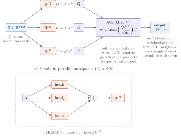
Transformer: mechanism diagram.
2. RoPE
RoFormer: Enhanced Transformer with Rotary Position Embedding. Su et al., Neurocomputing 2024.
Problem: Additive position vectors encode absolute position, though attention usually wants relative position. Find $f_q,f_k$ so that position enters the score only through the offset between tokens.
$$f_q(x_m,m)=R_{\Theta,m}W^Qx_m$$
$$ R_{\Theta,m}^\top R_{\Theta,n}=R_{\Theta,n-m}$$
$$ \theta_i=10000^{-2(i-1)/d}.$$
Shown:
- $R_{\Theta,m}$ is block-diagonal with $2\times2$ rotations by $m\theta_i$. The one-parameter group property, not orthogonality alone, gives $\langle f_q,f_k\rangle=q_m^\top R_{\Theta,n-m}k_n$.
- The paper derives an upper bound on the score whose position factor shrinks numerically over its plotted range.
My reading: Treat coordinate pairs as complex numbers and put $h=n-m$. The score is $\mathrm{Re}\sum_i\bar q_ik_ie^{\mathrm{i}h\theta_i}$, a trigonometric polynomial in the lag with content-dependent coefficients. For the same vector at both positions this is $\sum_i|q_i|^2\cos(h\theta_i)$, a stationary covariance with spectral measure $\tfrac12\sum_i|q_i|^2(\delta_{\theta_i}+\delta_{-\theta_i})$ (Herglotz, the integer-lag form of Bochner). For $q\neq k$ the lag function is positive semi-definite iff every $\bar q_ik_i\ge0$, which generically fails.
Consequence: the score cannot decay to zero. It is almost periodic in $h$. The paper’s decay claim concerns an upper bound examined numerically over a plotted range, not the score. This derivation is mine, not the paper’s.
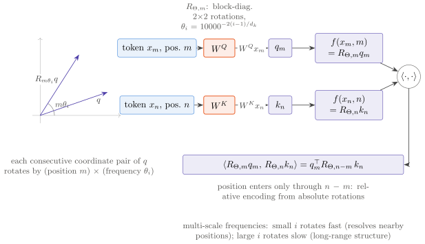
RoPE: mechanism diagram.
3. ViT
An Image is Worth 16x16 Words. Dosovitskiy et al., ICLR 2021.
Problem: Can a plain Transformer replace convolutions? Cut an image into $N=HW/P^2$ patches and treat them as tokens.
$$z_0=\big[x_{\mathrm{cls}};\,x_p^{(1)}E;\dots;x_p^{(N)}E\big]+E_{\mathrm{pos}}.$$
Shown:
- Large ViTs on ImageNet-1k alone trail ResNets without strong regularization, reach them with ImageNet-21k, and pass them with 300M-image JFT pretraining, measured after fine-tuning.
- Only the patchwise MLP layers are local and translationally equivariant. 2D structure is injected by hand only at patch extraction and position-embedding interpolation.
My reading: A bias–variance reading (mine; the paper’s phrase is “large scale training trumps inductive bias”): dropping most of the convolutional bias raises the data requirement. The result is about pretraining scale and is evaluated after transfer, not a statement that CNN priors are wrong.
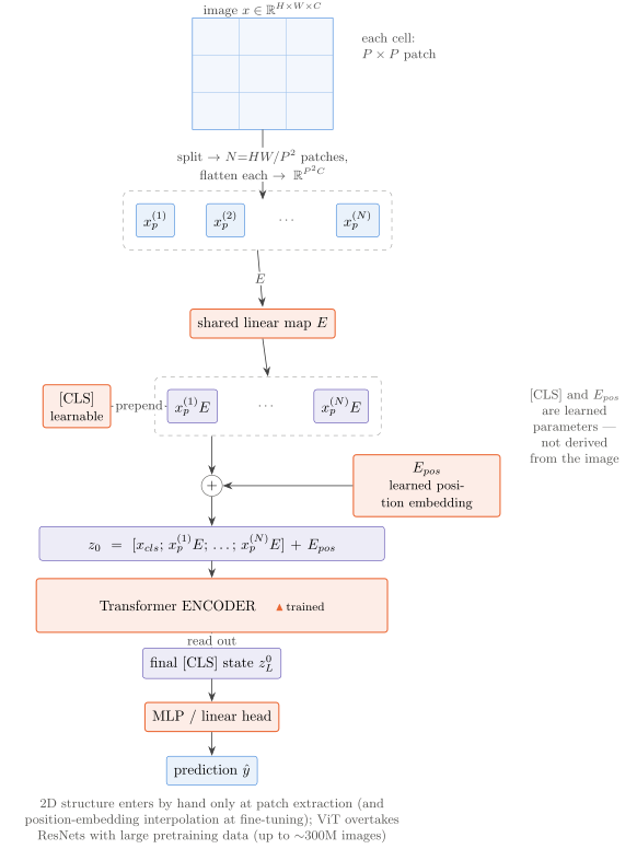
ViT: mechanism diagram.
4. BERT
Bidirectional Encoder Representations from Transformers. Devlin et al., NAACL 2019.
Problem: Pretrain a bidirectional encoder on unlabeled text. Conditioning on both sides needs an objective other than next-token prediction.
$$\mathcal{L}_{\mathrm{MLM}}(\theta)=-\mathbb{E}\sum_{i\in\mathcal{M}}\log p_\theta\big(x_i\mid\tilde x_{1:T}\big).$$
Shown:
- 15% of positions are selected; of those, 80% become [MASK], 10% a random token, 10% stay. The paper credits bidirectionality and its two pretraining tasks for most of the gain; pretrain-then-fine-tune already existed.
- Removing next-sentence prediction hurts QNLI, MNLI and SQuAD 1.1 in this paper. The finding that it is dispensable is later work, RoBERTa (Liu et al., 2019), with a changed input format.
My reading: The objective is composite-likelihood-style (Lindsay, 1988): a sum of conditional log-scores at randomly selected positions, each given the whole corrupted sequence, so it is not Besag’s pseudo-likelihood (Besag, 1975). Unlike Lindsay’s construction, the terms do not come from one parametric joint model, and the conditionals need not be compatible with any joint density. Hence no tractable generation.
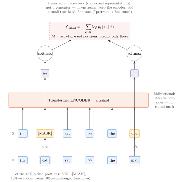
BERT: mechanism diagram.
II. Scale
5. GPT-3
Language Models are Few-Shot Learners. Brown et al., NeurIPS 2020.
Problem: How far does next-token prediction go at 175B parameters, and does in-context learning, weak in GPT-2, improve with scale?
$$\max_\theta\sum_t\log p_\theta(x_t\mid x_{<t})$$
$$\text{few-shot: }p_\theta\big(\cdot\mid(x_1,y_1),\dots,(x_n,y_n),x_{n+1}\big).$$
Shown:
- 125M to 175B parameters on about 300B tokens; the largest has $d=12288$ and 96 layers. Few-shot evaluation takes no gradient step.
- Validation loss follows a power law in training compute. The zero-to-few-shot gap often grows with capacity, which perhaps suggests larger models are more proficient meta-learners.
My reading: In-context learning is conditioning under a fixed distribution. The analogy to a posterior predictive is informal only: $\theta$ is a point estimate and there is no latent-task model. The paper’s own frame is meta-learning, and it stays explicitly agnostic on whether the model learns a task at inference time or recognizes patterns seen in training.
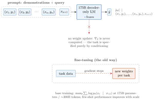
GPT-3: mechanism diagram.
6. LLaMA
Open and Efficient Foundation Language Models. Touvron et al., arXiv 2023.
Problem: For a target quality, training a smaller model for longer can lower inference cost. Test this past the usual ratio of tokens to parameters.
Shown:
- Sizes 7B to 65B on 1.0 to 1.4T public tokens, with pre-normalization by RMSNorm, SwiGLU, and RoPE.
- 13B outperforms 175B GPT-3 on most benchmarks, as the paper states, with exceptions such as PIQA. Training loss was still falling at the end.
My reading: Tokens per parameter from the paper’s Table 2: about 149 (6.7B on 1.0T), 77, 43, and 21.5 (65.2B on 1.4T), against the 20:1 baseline the paper quotes (“a 10B model on 200B tokens”). The comparison with GPT-3 is not controlled: architecture and data both differ, and baseline numbers come from the corresponding papers. So it does not isolate the effect of more tokens.
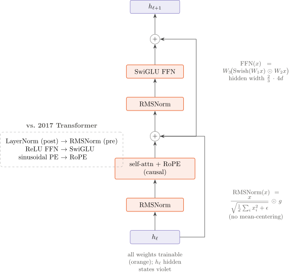
LLaMA: mechanism diagram.
7. MoE
Outrageously Large Neural Networks. Shazeer et al., ICLR 2017.
Problem: Grow parameters without growing the computation spent on each input, by routing each input to a few experts.
$$y=\sum_{i=1}^EG(x)_ie_i(x)$$
$$ G(x)=\mathrm{softmax}\big(\mathrm{KeepTop}k(H(x))\big).$$
Shown:
- Expert FLOPs scale with $k$, not $E$. The tunable noise in $H$ helps load balancing and supplies the smoothness that lets gradients pass through.
- Language models reached 131,072 experts (137B), but the best perplexity was at 65,536 (68B); 131,072 degraded. Translation used up to 2048 experts.
My reading: A covariate-dependent sparse combination in the Jordan–Jacobs mixture-of-experts tradition, which the paper cites for softmax gating. The form $\sum_i g_i\mu_i$ matches a mixture-of-experts conditional mean; what is absent is a mixture likelihood or latent indicator. The layer is a network component trained by backpropagation. The load losses are hand-weighted squared coefficients of variation across experts in a batch.
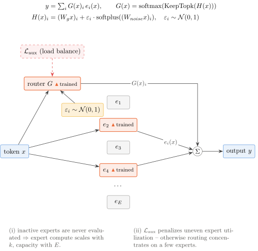
MoE: mechanism diagram.
III. Generative models
8. VAE
Auto-Encoding Variational Bayes. Kingma and Welling, ICLR 2014.
Problem: Fit $p_\theta(x,z)$ with continuous latents when the posterior is intractable and the data are large.
$$\log p_\theta(x)\ge\mathbb{E}_{q_\phi(z\mid x)}[\log p_\theta(x\mid z)]-\mathrm{KL}\big(q_\phi(z\mid x)\,\|\,p(z)\big)$$
$$ z=\mu_\phi(x)+\sigma_\phi(x)\odot\varepsilon.$$
Shown:
- Reparameterization turns the gradient into a pathwise expectation, replacing a naive estimator the paper reports as very high variance. The Gaussian KL is closed form.
My reading: Amortized variational inference: one network $q_\phi$ replaces per-datum variational parameters. (“Amortized” is the later word; the paper says recognition model.) Then $\log p_\theta(x)-\mathcal{L}=\mathrm{KL}(q_\phi(z\mid x)\,\|\,p_\theta(z\mid x))$ exactly, so the bound is tight iff the approximate posterior is exact.
The link to diffusion is narrower than often said: both use $z=\text{mean}+\text{scale}\cdot\varepsilon$, but diffusion’s forward process has no trainable parameters, so no pathwise gradient through sampling is needed.
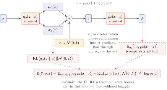
VAE: mechanism diagram.
9. GAN
Generative Adversarial Nets. Goodfellow et al., NeurIPS 2014.
Problem: Learn to sample without writing a likelihood: train a generator against a discriminator.
$$\min_G\max_D\ \mathbb{E}_{p_{\mathrm{data}}}[\log D(x)]+\mathbb{E}_{p_z}[\log(1-D(G(z)))]$$
$$ D^\ast=\frac{p_{\mathrm{data}}}{p_{\mathrm{data}}+p_g}.$$
Shown:
- With optimal $D$ the objective is $-\log4+2\,\mathrm{JSD}(p_{\mathrm{data}}\,\|\,p_g)$. Training alternates updates, and the generator in practice maximizes $\log D(G(z))$ to avoid saturation.
- The paper warns of “the Helvetica scenario”, later called mode collapse, and claims no sample-quality advantage over existing methods.
My reading: Where $p_{\mathrm{data}},p_g>0$, with equal class weights and at the optimum, $D^\ast/(1-D^\ast)=p_{\mathrm{data}}/p_g$, so $\mathrm{logit}\,D^\ast$ is the log density ratio: the discriminator is a classifier-based density-ratio estimator. The paper treats $D$ as maximum likelihood for $P(Y=y\mid x)$, not in these words.
The JSD statement is a non-parametric result. The paper says so itself: optimizing $\theta_g$ rather than $p_g$ means “the proofs do not apply”.
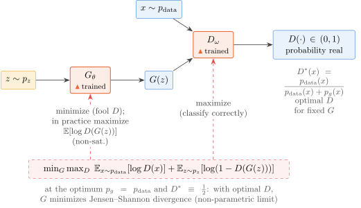
GAN: mechanism diagram.
10. Latent diffusion
High-Resolution Image Synthesis with Latent Diffusion Models. Rombach et al., CVPR 2022.
Problem: Pixel-space diffusion is expensive. Train a perceptual autoencoder, then run diffusion on the latent, with conditioning by cross-attention.
$$\mathcal{L}_{\mathrm{LDM}}=\mathbb{E}\,\big\|\varepsilon-\varepsilon_\theta\big(z_t,t,\tau(y)\big)\big\|^2$$
$$ z_t=\sqrt{\bar\alpha_t}\,z_0+\sqrt{1-\bar\alpha_t}\,\varepsilon.$$
Shown:
- Downsampling factors 4 and 8 work best. Savings are empirical, not a scaling law: 916 V100-days for ADM against 271 for LDM-4 and 79 for LDM-8 on ImageNet.
- The extracted paper text never mentions Stable Diffusion.
My reading: Denoising is score estimation. Under squared loss the optimum is $\varepsilon^\ast(z_t,t)=\mathbb{E}[\varepsilon\mid z_t]$, and since $z_t\mid z_0\sim\mathcal{N}(\sqrt{\bar\alpha_t}z_0,(1-\bar\alpha_t)I)$, Tweedie’s formula (Efron, 2011) gives $\nabla\log q_t(z_t)=-\mathbb{E}[\varepsilon\mid z_t]/\sqrt{1-\bar\alpha_t}$. The paper says only that its objective mirrors denoising score matching.
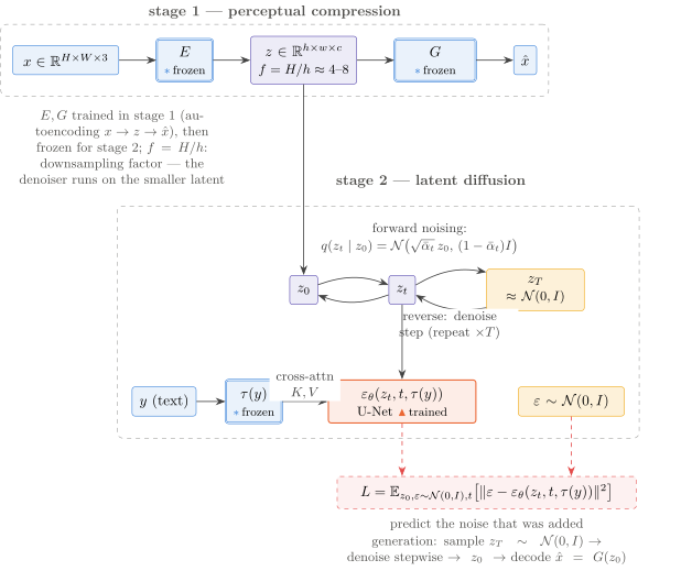
Latent diffusion: mechanism diagram.
IV. Adaptation
11. Adapters
Parameter-Efficient Transfer Learning for NLP. Houlsby et al., ICML 2019.
Problem: Share one frozen backbone across tasks by inserting small trainable modules.
$$\mathrm{Adapter}(h)=h+W_{\mathrm{up}}\,g(W_{\mathrm{down}}h)$$
$$ m\ll d.$$
Shown:
- Two adapters per Transformer layer; adapters, layer norms and the task head train.
- GLUE on BERT-large: 80.0 against 80.4 for full fine-tuning with about 3.6% of parameters and a per-task adapter size.
My reading: Adapters are a nonlinear residual bottleneck on activations; LoRA is linear in $x$ and bilinear in $(B,A)$, a reparameterization of a weight, so it can merge away. Both start at or near the pretrained model: approximately for adapters, exactly for LoRA with $B=0$.
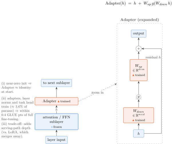
Adapters: mechanism diagram.
12. LoRA
Low-Rank Adaptation of Large Language Models. Hu et al., ICLR 2022.
Problem: Fine-tuning large models is costly in memory and storage. Freeze $W_0$ and learn a low-rank update.
$$h=W_0x+\frac{\alpha}{r}BAx$$
$$ B\in\mathbb{R}^{d_{\mathrm{out}}\times r},\ A\in\mathbb{R}^{r\times d_{\mathrm{in}}}$$
$$ B_0=0.$$
Shown:
- On the paper’s three GPT-3 175B tasks, $r$ as small as 1 to 4 on $W^Q,W^V$ matches full fine-tuning at about 0.003 to 0.01% of parameters. The authors do not expect this for every task.
- Evidence for low intrinsic rank is indirect: accuracy is nearly flat in $r$, and only the top singular direction of learned $A$ is shared between $r=8$ and $r=64$.
My reading: A reduced-rank parameterization of the update, in the spirit of reduced-rank regression (Izenman, 1975): $\mathrm{rank}(\Delta W)\le r$. When $B,A$ have full rank $r$, the factorization is identified only up to $(B,A)\mapsto(BG,G^{-1}A)$ for $G\in GL(r)$, so $\Delta W$ has $r(d_{\mathrm{in}}+d_{\mathrm{out}})-r^2$ free dimensions, not $r(d_{\mathrm{in}}+d_{\mathrm{out}})$. The paper does not state this.
The initialization is asymmetric for a reason the paper leaves implicit: $A=B=0$ is a stationary point, while at $B=0$ with $A\neq 0$ we have $\partial L/\partial A=0$ and $\partial L/\partial B\neq0$ in general, so $B$ moves first and both train after that.
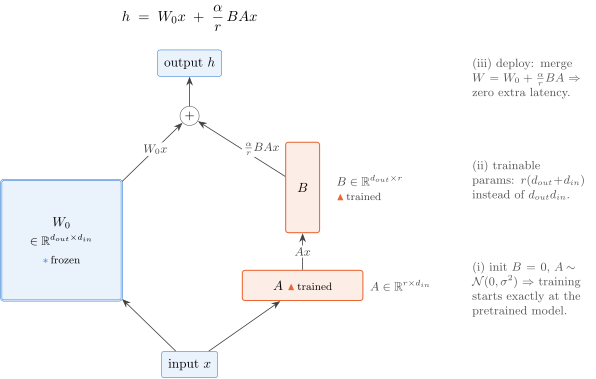
LoRA: mechanism diagram.
V. Knowledge and preferences
13. RAG
Retrieval-Augmented Generation for Knowledge-Intensive NLP Tasks. Lewis et al., NeurIPS 2020.
Problem: Combine a parametric generator with a non-parametric document memory, and train through the retrieval.
$$\text{Sequence: }p(y\mid x)\approx\sum_{z\in\mathrm{top}\text{-}k}p_\eta(z\mid x)\prod_ip_\theta(y_i\mid x,z,y_{<i}),$$ $$\text{Token: }p(y\mid x)\approx\prod_i\sum_{z}p_\eta(z\mid x)\,p_\theta(y_i\mid x,z,y_{<i}).$$
Shown:
- The query encoder and BART generator train end to end; the passage encoder and index stay fixed. Fine-tuning uses no passage labels, though the retriever starts from supervised DPR.
- The generator runs once per passage. The latent-variable idea existed for extractive QA; the contribution is extending it to general sequence-to-sequence generation.
My reading: RAG-Sequence is a finite mixture over retrieved passages with latent $z$, fitted by marginal likelihood with Adam, not EM. The components depend on $x$ through the top-$k$ set, and truncation is the stated approximation. The weights sum to one only if renormalized: the paper does not settle this, though the Hugging Face implementation does renormalize.
RAG-Token is exactly the marginal under $z_i\overset{\mathrm{iid}}{\sim}p_\eta(\cdot\mid x)$, one latent per token, since $\sum_{z_{1:N}}\prod_i=\prod_i\sum_{z_i}$. The two models coincide for length-one outputs.
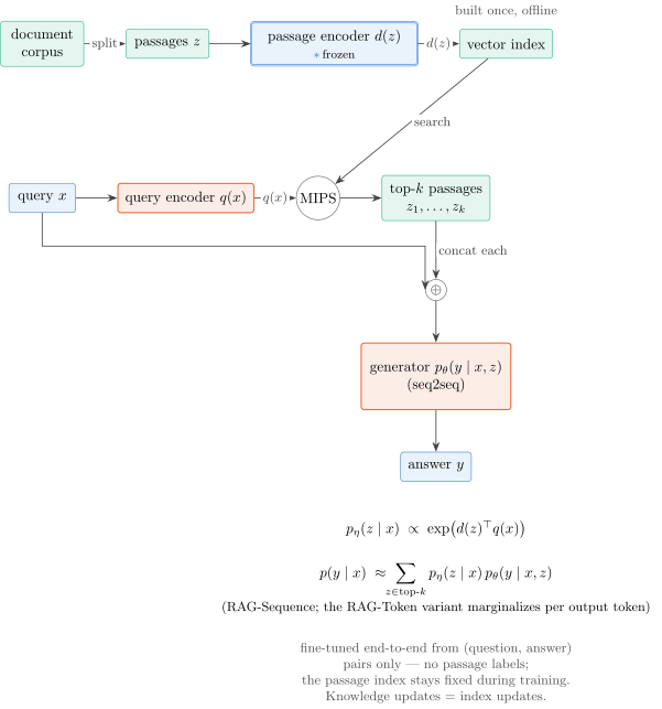
RAG: mechanism diagram.
14. RLHF
Deep Reinforcement Learning from Human Preferences. Christiano et al., NeurIPS 2017.
Problem: When no reward can be written down, learn one from human comparisons of behavior clips. The approach is older; the contribution is scaling it to deep RL.
$$\hat P[\sigma^1\succ\sigma^2]=\frac{\exp\sum_t\hat r(s^1_t,a^1_t)}{\exp\sum_t\hat r(s^1_t,a^1_t)+\exp\sum_t\hat r(s^2_t,a^2_t)}.$$
Shown:
- Policy training, human labeling and reward fitting run concurrently, with cross-entropy on the labels.
- About 900 queries, under an hour of the authors’ feedback, taught a simulated Hopper a backflip.
My reading: Bradley–Terry (Bradley and Terry, 1952) with log-strength equal to summed reward, $P(\sigma^1\succ\sigma^2)=\sigma(R_1-R_2)$. The fitted likelihood is the contaminated version $0.05+0.9\,\sigma(R_1-R_2)$.
The likelihood sees $\hat r$ only through differences of segment sums, so a constant shift cancels for equal-length segments; further invariances can exist, and $\hat r$ is constrained only on visited state–action pairs. The scale is relative to human choice noise, which the paper treats as arbitrary, normalizing $\hat r$ to a fixed standard deviation. Query selection by ensemble disagreement is similar in spirit to query-by-committee; the paper calls it crude and reports that it hurts on some tasks.
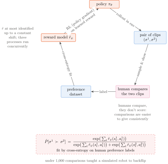
RLHF: mechanism diagram.
15. InstructGPT
Training Language Models to Follow Instructions with Human Feedback. Ouyang et al., NeurIPS 2022.
Problem: GPT-3 continues text rather than following instructions. Align it by supervised fine-tuning, then a reward model on human rankings, then PPO.
$$L(\psi)=-\mathbb{E}\big[\log\sigma\big(r_\psi(x,y_w)-r_\psi(x,y_l)\big)\big],$$ $$\max_\theta\ \mathbb{E}\Big[r_\psi(x,y)-\beta\log\frac{\pi_\theta(y\mid x)}{\pi^{\mathrm{SFT}}(y\mid x)}\Big]+\gamma\,\mathbb{E}\big[\log\pi_\theta(x)\big].$$
Shown:
- Raters preferred 1.3B InstructGPT to 175B GPT-3. Truthfulness improved overall, except that the 1.3B PPO-ptx model did slightly worse than a same-size GPT-3 model.
- The $\gamma$ term reduces, but does not remove, the alignment tax. Residual failures include false premises, over-hedging and multiple constraints.
My reading: The reward loss is logistic log-loss in the reward difference. That is Bradley–Terry in form, but the label is mine: the paper never names it. Pairs from one ranking are correlated, as the paper notes, so the sum is composite-likelihood-like rather than a ranking likelihood.
With $\gamma=0$ and $r$ fixed, $\max_\pi\mathbb{E}_\pi[r]-\beta\,\mathrm{KL}(\pi\,\|\,\pi^{\mathrm{SFT}})$ over all conditionals is solved pointwise in $x$ by the exponential tilt $\pi^\ast(y\mid x)\propto\pi^{\mathrm{SFT}}(y\mid x)\exp(r(x,y)/\beta)$, the Gibbs variational principle. The paper does not state this; a parametric policy under PPO only approximates it. So $\beta$ is a temperature.
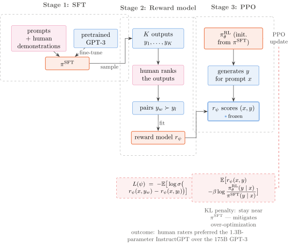
InstructGPT: mechanism diagram.
Threads
Where old statistics reappears:
- Paired comparisons: Bradley–Terry (1952) in RLHF, and in form in InstructGPT.
- Latent-variable marginal likelihood in RAG; amortized variational inference in VAE.
- Density-ratio estimation in GAN; score estimation through Tweedie in diffusion.
- Exponential tilting in the KL-penalized objective of InstructGPT.
- A spectral representation in RoPE, the reading closest to spatial statistics.
Where this lens stops: GPT-3 and LLaMA are mainly empirical findings about scale and engineering. I see no theorem underneath them, and these notes do not pretend otherwise.
What reading the source changed:
- RoPE’s score does not decay. A bound does, numerically, over a plotted range.
- BERT’s own experiments say next-sentence prediction helps.
- The largest MoE model was not the best one.
- Latent diffusion reports empirical savings, not a scaling law.
- GPT-3 says “often” and “perhaps” where summaries say “shows”.
References for the statistical readings
- Bradley, R. A. and Terry, M. E. (1952). Rank analysis of incomplete block designs: I. The method of paired comparisons. Biometrika 39, 324–345.
- Besag, J. (1975). Statistical analysis of non-lattice data. The Statistician 24, 179–195.
- Efron, B. (2011). Tweedie’s formula and selection bias. JASA 106, 1602–1614.
- Izenman, A. J. (1975). Reduced-rank regression for the multivariate linear model. Journal of Multivariate Analysis 5, 248–264.
- Lindsay, B. G. (1988). Composite likelihood methods. Contemporary Mathematics 80, 221–239.